Source Release of Cornflakes/Popcorn
Intro
I have released the source code of my new scientific packages, cornflakes and popcorn. They are located in Bitbucket repositories at
This package has been under development for the last two years as I’ve developed a variety of numerical codes. It is finally at the point where I am comfortable putting it out in the wild. It is still not quite ready for actual usage by people other than myself, but it is suitable as a case study in scientific package architecture.
The design goal for cornflakes/popcorn is to become a tool for implementing new numerical methods and the domain specific languages for them. The popcorn DSL is a transpiler for symbolic expressions, and cornflakes is an implementation of a general purpose map-assemble operator with supporting code for building hypergraph representations of problems.
The names are puns on “kernel”: Cornflakes is the serial assembly of kernels. Popcorn transforms compact kernel specifications in large and fluffy C code implementations. Husks are filled with kernels. (Cornflakes will run in parallel though, but I still liked the pun.)
Overview
In the design philosopy of cornflakes, many high performance scientific programs all share a similar characteristic:
- Calculations are performmed on a small chunk of data at a time: the physical kernel. (This is the realm of popcorn.)
- The inidividual calculations and required data are distributed across a large amount of resources for parallel computation. (This is the realm of cornflakes.)
For a finite element method program, the calculation of the local element matrix is the kernel that is the smallest unit of computational work to be distributed across processing nodes. Developing algorithms and working code on both sides of the program is a challenge.
Higher order numerical algorithms for both temporal discretizations, such as many-stage implicit Runge-Kutta methods, and spatial discretizations, such as high order finite element basis functions, are, in the author’s opinion, underused owing to the great difficulties in their implementation. A major barrier to using the more complex numerical schemes is the generation of the tangent matrix: that is, the $\mathbf{K}$ in the problem $\mathbf{K}\mathbf{u}=\mathbf{f}$. Developing the form of the matrix is manageable for linear problems, though quickly becomes difficult for nonlinear fully-coupled multiphysics problems. These types of problems are typically described mathematically as either minimization problems on a Lagrangian or some other expression of a potential, \begin{equation} \min_{\mathbf{u}}\Pi\left(\mathbf{u}\right), \end{equation} or as nonlinear systems of equations, \begin{equation} \mathbf{f}\left(\mathbf{u}\right)=0. \end{equation} Solving these problems statically or with an implicit time stepping method usually centers around linearizing the functions and employing Newton’s method, or some variant thereof, and iterating over a series of linear systems, \begin{equation} \mathbf{f}\left(\mathbf{u}^{I}\right)+\left.\frac{\partial\mathbf{f}}{\partial\mathbf{u}}\right|_{\mathbf{u}^{I}}\Delta\mathbf{u}^{I} = 0, \end{equation} with $\mathbf{f}=\frac{\partial\Pi}{\partial\mathbf{u}}$ if the problem was originally expressed with a potential. Even neglecting the effort required to write the code itself, it can require many weeks of pencil-and-paper work manipulating the mathematical expressions to produce a linearized equation.
The Readme.md in the cornlakes repository explains the hypergraph and map-assemble abstraction in great detail. In the rest of this post, I talk about a very complicated example that motivated its development, and then some software design considerations I am still mulling over.
Example
See the example notebook in the repository, /examples/spring_example.ipynb
Usages
Cornflakes the main library for a number of different of codes I write at LBNL. The following publications and conference presentations are a small selection. The poster has a good description of the algorithm that was possible using cornflakes.
- Queiruga, A. F. and G. J. Moridis, “NG21A-1806: Numerical Simulation of Hydraulic Fracture Propagation using Fully-Coupled Peridynamics, Thin-Film Flow, and Darcian Flow”, AGU Fall Meeting, San Francisco, CA, December 2016. (poster linked)
- Queiruga, A. F. and G. J. Moridis, “Numerical experiments on the convergence properties of state-based peridynamic laws and influence functions in two-dimensional problems.” Computer Methods in Applied Mechanics and Engineering 322 (2017): 97-122.
- Moridis, G. J., A. F. Queiruga, and M. T. Reagan, “The T+H+M Code for the Analysis of Coupled Flow, Thermal, Chemical and Geomechanical Processes in Hydrate-Bearing Geologic Media,” 9th International Gas Hydrates Conference, Denver, CO, June, 2016.
Consider the follow diagram of the simulation for hydraulic fracture extension described in the above poster:
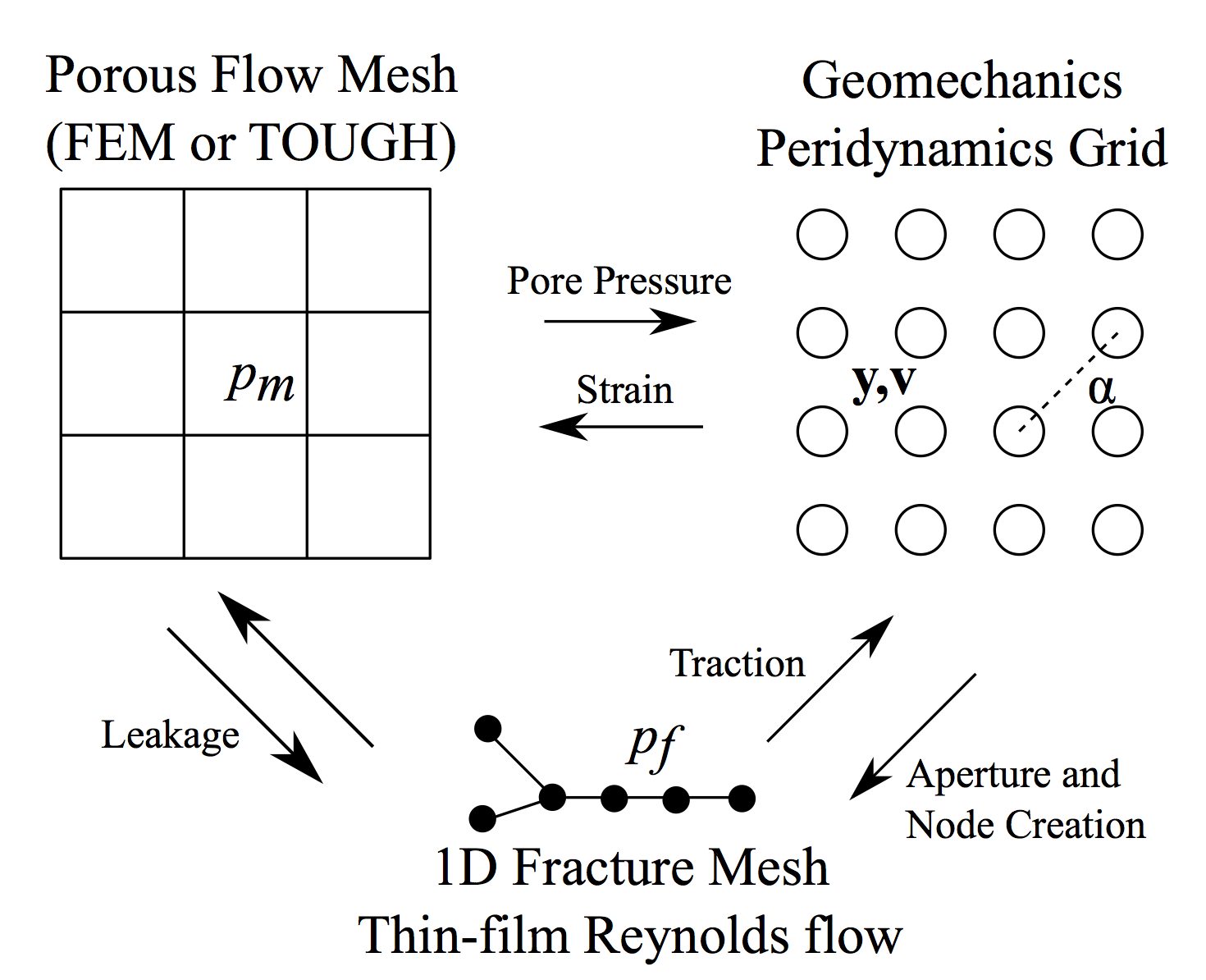
It involves three different types of discretizations for three different sets of physics:
- a Peridynamics grid for mechanics and fracture,
- a 2D Finite Element mesh for porous flow, and
- a 1D Finite Element mesh for fracture transport that’s dynamically remeshed
that are fully coupled. A visualization of the simulation is included in the research gallery on this slide, and the poster linked above describes the algorithm. How does one even program this? Well, it took me less than a year because, in that time, I wrote my own langauge and runtime to express it with! Using cornflakes, there are three classes of hypervertices in this problem:
- Peridynamics points, $P$
- Peridynamics bonds, $B$
- Background mesh nodes, $Q$
That model overview can be decomposed into the following (hand drawn) kernels:
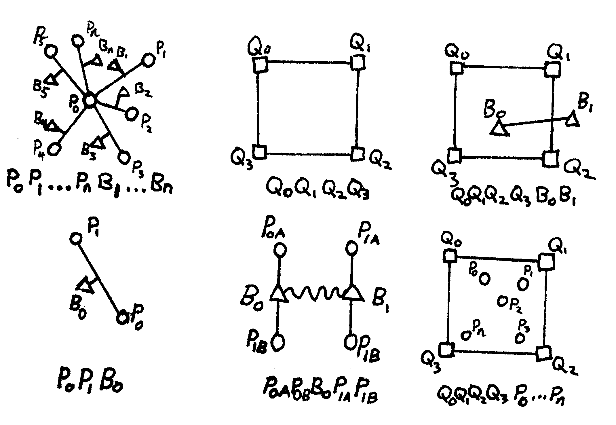
The schematic illustrates the physical meaning of the edge, and the bottom list shows the ordering of the hypervertices inside the hyperedge that corresponds to one kernel call. From left to right, top to bottom, these are
- For state-based peridynamics: A point with vertex id $P_0$ surrounded by points with ids $P_1$ to $P_n$, connected with bonds who themselves have vertex ids $B_1$ to $B_n$;
- For Darcy flow with FEM: A simple four-node quad whose nodes are vertices $Q_0$ to $Q_3$;
- For fracture-matrix leakage connected a four node quad with a line segment: The four-node quad ($Q_0$ to $Q_3$) PLUS a two-node line, $B_0$ and $B_1$;
- For damage evaluation: A single bond $B_0$ between points $P_0$ and $P_1$;
- For fracture flow: A line segment FEM connecting the bonds $B_0$ and $B_1$, which is directly coupled to the four peridynamics points defining the bond; and
- For poroelastic (porous flow to mechanics) coupling: A quad with a set of points inside of it.
The vertex ids are just integers, with $P$, $B$, and $Q$ just denoting different ranges. E.g., if there are 100
peridynamics points, 800 bonds, and 40 fem nodes, the last vertex has the id 939. The ranges would be 0-99 for $P$,
100-899 for $B$, and 900-939 for $Q$. The labels mean absolutely nothing to cornflakes, but we use these types
of schematics to figure out what the DofSpaces and DofMaps need to look like to fetch the data we need for
each kernel. Note that the first and last kernel are variable length! The edges of a hypergraph don’t require the
same length, and popcorn kernels can take in variable length arguments, given an l_edge parameter, and the
DSL can express Loops over symbolic ranges.
Stylistic Choices
Language
I chose Python/C because it was, and still is, the state of the art when I started writing. At the time I began, I felt that Julia wasn’t quite ready. Originally, I wanted cornflakes to have a pure C API that didn’t require Python to make it easy to link to preexisting code. Julia requires the runtime and doesn’t support outputting linkable objects, but I have abandoned that decision and am okay with that now. The latest version of TOUGH+ has an embedded Python interpreter that executes the Python/C-based mechanics library
Julia also has a very good macro system, enabling manipulation of the AST. I want to implement Popcorn inside of Julia entirely, instead of the Python–>C generation scheme. However, Julia doesn’t have its own symbolic library, and the Python interface was wonky when I experimented with it. I think it would be possible to use Sympy inside of Julia now, but there are still two languages. Sympy is slow for some of my calculations, too. Maybe a new symbolic toolkit in Julia that leverages its JIT could be blazingly fast.
C Api
I wanted a pure C API at first, but this gets out of hand quickly. Just embed a higher level language when you need to interact with legacy codes. It’s easier than expressing complicated simulations in pure C or Fortran.
Integrating parallelism in a prototyping environment.
At first I wanted a serial and a parallel implementation of the runtime; i.e. one for interactive runs in IPython on a laptop and one for HPC systems. (Hence the “cereal” pun for cornflakes. The parallel version was going to be called cornfield or thresher or some other pun involving many stalks of corn.) However, I think it’s best to only have one version. Requiring the user to install PETSc for a laptop system also can complicate matters. Distributing Docker images solves the problem of requiring HPC libraries, so it may be viable to require a PETSc backend. However, I am still conflicted on how to manage the type system to make the Numpy/Scipy types transparent, but still wrap parallel data structures. I think the Julia array interface would solve this, but that may be wishful thinking.
SWIG
I used SWIG as the Python/C binding since it’s worked well enough for me in the past. I probably won’t use it again. This has caused tons of headaches with allocation tracking and memory leaks. I even had to make direct calls to the Python API.
Object system
If you look carefully at the C source, you’ll notice that I hand-coded my own polymorphic object system for
cfdata_t, cfmat_t, and dofmap_t.
Don’t do this! This is bad practice! I’m a crazy person!
I would never use an obscure practice in a codebase with multiple authors.
General purpose software should avoid using motifs only familiar to low-level C programmers to remain accessible to
the users; a cryptic implementation won’t be educational to an end user trying to learn more about the software design.
I just really hate the C++ class system, but that’s another discussion about language design.
(My latest C++ code has a hacked vtable, too, for virtual template methods.)
I really like the Julia type system, which is another motivator for switching.
Some of the blame goes to my colleague Jeff Johnson, who may have been a bad influence on that. (He points out that this paradigm is indeed very common, to which I counter that, unlike us, most fellow scientists don’t spend their free time reading the Linux kernel source for inspiration.) I jest; I thank him dearly for our discussions on code architecture for these types of packages. Cornflakes would have been much messier without his advice.
Acknowledgements
Besides the excellent advice from Jeff mentioned above, there were a number of important inputs to my line of tought. The FEniCS project is a central inspiration to this work. My frequent discussions (or arguments) about DSLs with Daniel Driver, author of “Dan++”, yielding many design decisions to cornflakes. I also acknowledge the inspiration of Per-Olof Persson, whose one line in a lecture on Runge-Kuttas six years ago—“You just implement $\mathbf{u}$ as a pointer to data”—completely changed my view of what the right data structures should be.
Development support for this language was provided while addressing the needs of multiple projects at Lawrence Berkeley National Lab, including those mentioned above.
Future
Cornflakes was designed as a new way to express parallelism, but I still haven’t done it.
The unstructured hypergraph partitioning algorithm has been implemented and tested in another development code
using PETSc, but hasn’t made its way into cornflakes yet.
I am still debating on the major type system changes I discussed above before parallelizing cornflakes.
A deprecated implementation is in the source code for OpenMP threading of Assemble.
The popcorn specification should also be able to generate code for vectorized CPUs and GPUs quite easily.
I will be soon adding a more complex example of a family of meshless methods (Moving Least Squares and the Reproducing Kernel Particle Method) to the cornflakes repository. I am also preparing an open source Peridynamics solver based on cornflakes to be released ahead of some upcoming conference presentations.
I’ll probably be rewriting it all in Julia at some point.